Megakernels on Mac: What Fusion Saves and What It Costs
Persistent workers, memory reuse, and the dependencies that survive fusion. Why an improved megakernel still lost to optimized separate kernels.
 Written by Abhishek Gahlot
The goal was a 27-billion-parameter model running fast on one Mac: 200 tokens per second on 5K–10K-token coding prompts, ahead of Splash and MLX. A megakernel seemed worth trying because it could keep more work on the GPU and remove boundaries between operations. After weeks of work, the improved prototype was still 2.7% slower than optimized separate kernels.
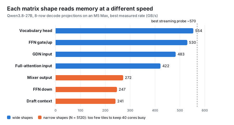
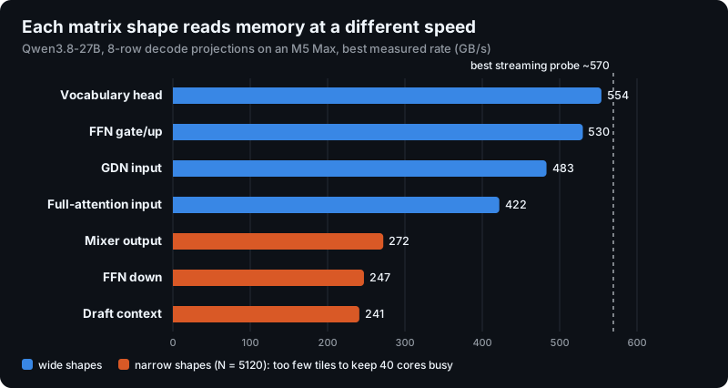
The difficulty was inside those operations. The M5 Max streaming probe reached roughly 570 GB/s, but some important projections used less than half that rate.
The work behind a token
A token is a piece of generated text. Producing it sends data through the model's projections, attention and recurrent layers. Each kernel is a GPU program responsible for part of that work.
Bandwidth measures how quickly data moves through memory. The audited execution path contained about 14.43 GB of target projection weights, plus draft and context projections, for 15.76 GB of logical payload. Moving that payload at 570 GB/s takes about 27.65 ms.
That gives the memory movement a useful scale. It does not make the difference between 27.65 ms and a roughly 40 ms cycle disposable: the cycle also performs arithmetic, updates state and waits for dependencies.
The chart shows another problem. FFN gate/up projections reached 530 GB/s, while FFN down reached 247 GB/s. FFN means feed-forward network. Both operations read quantized weights, but their matrix shapes give the GPU different amounts of parallel work. Removing the boundary between them does not automatically give the narrower operation a better schedule.
One submission, several kernels
A command buffer can submit several kernels together. Fusion goes further: it combines operations inside one kernel, allowing a worker to reuse a value before writing it to memory.
One submission in both cases. Different intermediate storage.
Three separate kernels
The buffer batches commands; intermediates cross dispatch boundaries.
One fused kernel
A worker carries its local value through the operations.
A persistent megakernel keeps workers alive across multiple stages. A scheduler assigns work as inputs become ready, instead of ending one dispatch and starting another.
The prototype joined FFN normalization, gate/up and down projections, then normalization and the next Gated DeltaNet input projection. Gated DeltaNet, or GDN, is the model's recurrent linear-attention mixer. Its scan followed that projection.
Produce. Two of four illustrative vector parts are ready. Normalization is blocked in both arrangements until every part is available.
Conceptual sequence. Playback timing is for explanation, not a benchmark. Use Step to read at your own pace.
The dependencies remain
After the down projection, root-mean-square normalization needs the sum of squares across the whole hidden vector. A worker finishing one quarter cannot normalize it using an unfinished sum. Fusion changes where partial sums live and how workers signal completion; the remaining quarters still have to finish.
Recurrence has the same constraint. If the next state is , the next token depends on the previous state. Independent state columns can run in parallel, but the token updates retain their order.
A persistent schedule now has to coordinate these dependencies itself. Queues, completion flags and barriers consume resources. Workers waiting for another stage can also occupy space that stage needs. A threadgroup barrier only coordinates its own group; it cannot safely replace a whole-grid synchronization scheme.
What the prototype lost
The captured FFN-to-GDN-input window took 521.2 µs, with only 7.7 µs between its kernels. Most of the time was already inside the operations.
The persistent worker arrangement suited some projections better than others. Leaving the input projection as a separate native kernel recovered roughly half a millisecond, but the hybrid still lost. Improving the full prototype made it 1.045% faster than its predecessor and 2.701% slower than optimized stock.
The worker timeline made the scheduling problem visible. In the instrumented run, 24 of 160 workers waited about 205 µs on early down-projection tickets while gate/up work finished. Other workers were busy during that wait. The average idle time was about 85 µs per worker, which is useful for locating imbalance, not a block of time that could all be recovered.
Extra staging did not help either. Loading down-projection weights through threadgroup storage added 20.714 µs with one slot and 22.670 µs with two-slot lookahead. Both variants lost all 24 pairs.
Register pressure was a plausible explanation for the broader regression. A better control produced paired medians of +0.043 and -0.044 ms/step, with no repeatable penalty and no reported spills. The earlier register attribution was withdrawn.
A stronger baseline changes the result
Lithos's GDN study exposed a similar distinction. Its optimized fused configuration took 599.72 µs, down from 646.25 µs. But the matched packed, separate-dispatch control took 596.02 µs. Packing and projection geometry supplied much of the improvement.
That distinction changes where the next effort belongs. A deeper K split brought one dependent-call down-projection probe from 118.8 to 99.7 µs, but changed output by about one BF16 unit in the last place. The short-K output projection got slightly worse. Shape, arithmetic and the required numerical behavior all affect which changes are usable.
The practical fusion boundary is the one that removes a specific read, write or repeated transformation without slowing the surrounding work. Existing primitives in Metal Performance Shaders, Metal Performance Primitives or MLX may already do the job. Larger fused regions need to earn the extra coordination they introduce.
The other route toward 200 tok/s is more useful output from each target pass. That leads to drafters and speculative decoding, then the complete Pulsar results.
Methods and measurements
Bandwidth and memory measurements
The useful starting point is how much data the selected execution path moves, and which part of that movement fusion can remove. These experiments separate an observed streaming rate, a source-derived payload estimate, and the time spent between real kernels.
| Finding | Result | Evidence type | Interpretation |
|---|---|---|---|
| Best streaming configurations on the M5 Max | 563.7, 570.2 and 572.5 GB/s | Measured, three 4 GiB probe runs | Roughly 570 GB/s in this finite access-pattern and geometry sweep |
| Ordinary B1 projection payload | 15.758 GB | Calculated from a pinned model layout and call graph | Logical target, draft and context projection bytes; not measured DRAM traffic |
| Payload transferred at 570 GB/s | 27.65 ms | Conditional calculation | Reference transfer time if that logical payload crosses the interface at that rate |
| Internal gaps in an FFN-to-GDN-input window | 7.7 µs of 521.2 µs | Measured profiler window | Visible gaps were a small part of this region; producer and consumer work also occupied the kernel intervals |
The streaming probe swept three access patterns, four grid sizes and two threadgroup sizes. Each number above is the best configuration in its run, rather than a repeated sample of one fixed configuration. An older 8 GiB probe reported 512.9 GB/s, showing how strongly the access pattern and probe geometry can affect the result.
The saved streaming receipts do not record a sustained warm-up duration or a thermal plateau. They support an observed bandwidth reference, not a validated warmed maximum. A separate staging fixture recorded 3.02329 accumulated GPU seconds of warm-up outside its timing window; that preparation applies to that fixture alone. Measurement notes and source receipts
The 27.65 ms estimate
The projection audit counted 14.434467840 GB of target payload and 1.323417600 GB of draft and context payload. The target feed-forward gate/up/down subset accounted for 9.625927680 GB. The restricted draft head already includes its mutable segment, so it is counted once.
This calculation prices a particular logical payload at a particular reference rate. Cache reuse, repeated reads, discarded drafting, context length, model format and the selected graph can change actual traffic. A rigorous lower bound would need both a minimum amount of traffic across the limiting interface and an upper bound on its sustained service rate. The best observed streaming result establishes neither for every future design.
Subtracting 27.65 ms from a measured 40 ms cycle therefore does not identify 12.35 ms of removable overhead. The remainder includes computation, state and cache traffic, and dependencies. Those costs can overlap. Fusion needs a specific read, write or scheduling boundary to remove, rather than a gap between two numbers measured at different scopes.
The distinction between GPU warm-up, sustained heat and cache residency is covered in Pulsar's operating-condition measurements.
Projection shape changes the achieved rate
The streaming reference does not predict every matrix operation. An eight-row projection sweep reported the following best payload rates:
| Projection | Reported rate |
|---|---|
| Draft context | 241 GB/s |
| FFN down | 247 GB/s |
| Mixer output | 272 GB/s |
| Full attention input | 422 GB/s |
| GDN input | 483 GB/s |
| FFN gate/up | 530 GB/s |
| Vocabulary head | 554 GB/s |
The spread makes shape-specific controls important. A deeper K split reduced a dependent-call FFN-down probe from 118.8 to 99.7 µs, but changed results by about one BF16 unit in the last place. The short-K output projection instead moved from 36.7 to 37.3 µs, and independent-call timings were approximately unchanged. The numerical difference matters for byte-identical paths; the benefit also depends on the projection shape and call ordering. Projection and control receipts
Results from the persistent prototype
The measurements cover three levels: a captured kernel window, isolated projection variants and a paired serving comparison.
Small gaps between dispatches
In one captured FFN-to-GDN window, the separate-kernel path took about 521.2 microseconds. Approximately 7.7 microseconds lay between its kernels.
That is about 1.5% of that window. It does not mean all 7.7 microseconds can be removed, and it is not a full serving-cycle measurement. It establishes that the visible gaps were a small part of this particular region.
The producer's final work and the consumer's initial work also take time inside their kernel intervals. That work remains even when the dispatch boundary disappears.
Projection geometry and the persistent schedule
Different projections needed different amounts and shapes of parallel work. One persistent worker arrangement did not suit all of them.
Keeping the input projection as a native kernel recovered roughly half a millisecond in a hybrid experiment. The hybrid still did not beat the separate-kernel baseline.
An improved persistent prototype was then compared with both its predecessor and stock execution:
| Comparison | Observed result |
|---|---|
| Improved megakernel versus original megakernel | 1.045% faster |
| Improved megakernel versus optimized separate kernels | 2.701% slower |
This was a September 27 screen on Qwen3.8-27B, with three sampled seeds at each of 1K, 5K and 10K input lengths. The ratios were geometric means over nine paired comparisons; output hashes and useful-token counts matched. Each request had representative GPU warm-up. The metric was decode output tokens divided by the engine's recorded decode wall time, not latency to a completed answer.
Scheduling and synchronization costs
Instrumentation exposed costs hidden by the dispatch count. In one worker-timeline experiment, the separate chain took 407.6 µs, the persistent kernel 428.0 µs, and the instrumented persistent kernel 450.7 µs. The software clock itself added 5.3%, so its worker timings describe the instrumented run.
| Diagnostic | Recorded result | Measurement boundary |
|---|---|---|
| Early down-projection tickets | 24 of 160 workers waited about 205 µs while 136 gate/up jobs occupied one wave | Instrumented worker timeline; other workers were computing |
| Average worker idle time | About 85 µs per worker, including readiness waits and the final partial wave | Worker occupancy accounting, not 85 µs of recoverable critical-path time |
| In-kernel RMS normalization | Approximately 3.1–4.3 µs more per transition for the tested multi-worker variants | Three 24-round invocations against a matched down-kernel control followed by separate RMS normalization; Chrome open |
| Lean persistent variant versus stock | +4.55 µs/transition with Chrome closed; +4.97 µs/transition with it open | Separate direct-pair cohorts of 672 and 432 rounds; no causal Chrome comparison |
These diagnostics cover different variants and cannot be added into a single explanation of the serving regression. They show why removing a dispatch is insufficient: work distribution, readiness signalling and normalization can cost as much as the boundary they replace. The worker clock also perturbs execution, and average worker idle time can overlap useful work elsewhere. Diagnostic receipts and scope
Threadgroup staging
Two further variants loaded Q4 down-projection weights through threadgroup storage.
Across 24 alternating pairs, the one-slot version added about 20.714 microseconds per projection, and the two-slot lookahead version added about 22.670 microseconds. Neither won a pair.
These operator measurements used real weights and synthetic activations. Both tested implementations lost; the result does not generalize to every staging design or isolate occupancy as the cause.
The extra copies, synchronization and resource use must be repaid by the reuse they enable.
Register pressure remained unproven
The megakernel used more registers in the driver metadata, so register pressure was an attractive explanation.
A later control tried to match the extra loads and arithmetic while changing value lifetimes. Direct paired medians were +0.043 and -0.044 ms/step, without a repeatable penalty, and the inspected kernels reported no register spills. The control was imperfect, but it was enough to withdraw the earlier numerical attribution.
Saved frame-level counters reported approximately 15.5% and 18.0% occupancy, while active-core counters reported approximately 92.0% and 95.3%. These measure different things; low occupancy alone did not establish idle cores. Neither observation established the cause of the loss.
Packing and geometry in the unfused control
Lithos's published GDN study provides a useful independent example:
| Implementation | Reported mean of per-layer minimum times |
|---|---|
| Original implementation | 646.25 microseconds |
| Optimized automatic configuration | 599.72 microseconds |
| Matched packed multi-dispatch control | 596.02 microseconds |
| Independently tuned packed control | 598.87 microseconds |
The study attributes substantial improvement to operand packing and projection geometry. Fusion did not establish an advantage over the corresponding packed controls. These were fixed eight-row layer measurements, not generation throughput, and numerical equivalence to the original model was evaluated with tolerances. Author's study
Choosing a fusion boundary
A useful candidate removes identifiable work: an intermediate read/write, redundant transformation, repeated weight load or measured scheduling gap. Existing primitives in the runtime, Metal Performance Shaders (MPS), Metal Performance Primitives (MPP) or MLX may already cover it. When a new implementation needs better packing or tile geometry, the separate-kernel control needs the same improvement for the comparison to isolate fusion.
The numerical requirement also determines which changes are available. Byte equality, a documented tolerance, target-distribution preservation and task quality require different checks. A narrow candidate with explicit supported shapes and failure behavior is easier to validate against that requirement, including a case that breaks its central assumption. Operator measurements then feed into graph, stateful-model and serving tests before the implementation expands.
Fusion changes the cost of a target pass. Speculative decoding changes the useful progress obtained from it; Pulsar's engine measurements cover both in the complete serving path.
Further reading
Scheduling and correctness
Inside the persistent kernel, a compiler or hand-written scheduler describes which tasks exist, where their inputs live, and when they can run.
Conceptually:
while there is work in this region:
    obtain a task whose prerequisites are satisfied
    compute the task's output
    make the output visible to its consumers
    publish completion
This scheduling sketch leaves the synchronization unresolved. A Metal implementation needs a safe way to detect completed prerequisites and make their writes visible to consumers.
There are several reasonable fusion boundaries:
| Boundary | Possible benefit | New responsibility |
|---|---|---|
| Elementwise chain | Remove an intermediate read/write | Preserve operation order and tails |
| Projection plus epilogue | Reuse an accumulator before storing | Preserve reduction and rounding |
| Attention or GDN mixer | Reuse local statistics, state slices and layouts | Coordinate dependent tasks |
| Decoder layer | Reduce more boundaries | Accommodate very different stages |
| Whole decoding step | Keep the entire schedule on the GPU | Handle broad synchronization, state and resource lifetimes |
Larger regions offer more reuse, but also bring more varied work under one schedule.
For example, a layer's multilayer perceptron (MLP) might already have a very effective matrix kernel. Pulling it into a persistent worker layout can make that matrix operation slower even if the surrounding dispatch count falls.
An indirect command buffer, or another form of pre-encoded replay, addresses a different problem. It can reduce repeated host encoding work while preserving multiple GPU dispatches. An engine can use both command replay and mixer megakernels.
Dependencies and synchronization
After a down projection produces a hidden vector, root-mean-square (RMS) normalization needs the sum of squares of all its elements. A worker that finishes the first quarter must still wait for the remaining quarters before the final normalization factor is available.
Fusion can change where the partial sums live and how workers signal completion. It cannot generally normalize using an unfinished sum and remain equivalent.
The same principle applies to recurrence. If a state update is:
the next token's update depends on the previous state. Parallelizing independent state columns may help. Simply launching all token updates simultaneously does not preserve the recurrence.
Worker queues, completion flags and software barriers add coordination costs. A worker arrangement that suits one projection may undersupply another. A threadgroup barrier is not a whole-grid barrier, and a grid whose resident workers spin for unscheduled producers can fail to make progress.
The implementation must specify which worker owns each value, when writes become visible, and what happens on timeout or cancellation. Buffers cannot be released while submitted work can still read them. The next consumer must see the logically committed state, even if materializing that state was deferred.